Wave Functions of an Electron on a String and EM transitions

The electron on a string is one of the simplest models where the basics of quantum mechanics can be demonstrated. Unfortunately in high school one can use only real functions, which immediately causes some problems if one tries to answer some of the questions of a smart and interested student. Some of these “difficult” questions are the following:

• The wave function is usually represented as vibrations of a string. The square of the wave function shows “where” the electron is located (finding probability distribution). However, during the vibration there are moments when the displacement of the string is zero everywhere. Where is the electron in such a moment? Has it disappeared?

• The oscillation frequency of the wave function is known: E=h∙f. If the electron is oscillating like this, it should radiate energy like an antenna. Why electrons do not radiate in the eigenstates of the atoms, if their wave functions are oscillating? (The usual answer is that the electrons are “standing” still, only the wave function is oscillating.)

• How can one imagine that the wave functions are oscillating, but the electrons are standing?

• How can an electron emit or absorb electromagnetic radiation? Does it behave like an antenna? How can it do that, if it stands still in all atomic states?

This simulation gives some hints to understand these phenomena and to answer these questions.

Short theoretical summary

According to the quantum mechanics the wave function of an electron on a string is the following: .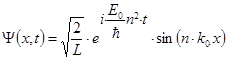

Itt , ,

L is the length of the string, m is the electron mass, and n = 1, 2, 3, 4… are the quantum numbers of the state.

Obviously, one cannot write down complex functions in high school! Instead, we can say that the state of a particle will be described by two (real) functions. Let us denote them Reѱ and Imѱ. These can be imagined as components of a vector. Then the (Reѱ)²+(Imѱ)² expression shows where the particle can be found. This might seem familiar also to students in high school, since they learned already how to calculate the length-square of a vector: by adding the squares of its components.

It is easy to see from the above complex expression that

, and .

This simulation helps to show the following:

1) To illustrate the two components of the wave function (Reѱ and Imѱ ), including their time behavior. Their frequency can be calculated as , where . This „illustration” can be done by drawing the real (Reѱ) and the imaginary part (Imѱ) separately (2D drawing), but it is also possible to draw them in a 3D coordinate system (x, Reѱ, Imѱ) .

2) It is also possible to draw a wave function composed as a superposition of two arbitrary selected wave functions.

The drawing can be performed as well in 2D as in 3D.

3) The simulation shows also the time and space behavior of the finding probability of the mixed state, as well as the position of its „center of mass”.
(The finding probability of one single state can be seen, if one “mixes” the same state.)

It is interesting to observe

a) The wave functions of the eigenstates are oscillating, but the distributions of their finding probabilities as well as their centers of mass are constant. Therefore the electrons in these states are not “moving”, therefore they do not radiate.

b) The center of mass of certain “mixed” states is oscillating. According to the electrodynamics an oscillating electrical charge (electron) radiates like an antenna.

c) It can be observed that the oscillation frequency is , i.e. the difference of the two original frequencies. (Please note that the amplitude and the frequency of the oscillation will be determined by the simulation, analyzing the resulting motion of the center of mass, and not using the above formula! Therefore one should wait a few oscillations until the correct amplitude and frequency will be shown.) Using the formula we get . This is Bohr’s result for the frequency of the emitted photon.

d) It can be seen, that only those superpositions lead to an oscillation of the center of mass, where the symmetry of the two components are different. There is no oscillation for
n = 1 and n = 3 mixture, or for the n = 2 and n = 4 mixture. This is the reason (in the case of the 3D atoms) that there is no photon emission at a 2s → 1s decay (since both quantum states are spherically symmetric, therefore the center of mass does not change at their mixture).